Subsections
Ordalie contains a collection of tools that can be called at any time, and that can stay alive whatever happens in the main window. It is necessary to leave a tool before using a new one.
4.1 Snapshot Overview
The 'Snapshot Overview' is one of the available schematic representation of a snapshot. When launched, a window appears with the schematic snapshot at the top and a control panel at the bottom. Any number of Overviews can be launched for a given snapshot.
Figure 3:
The Overview tool window
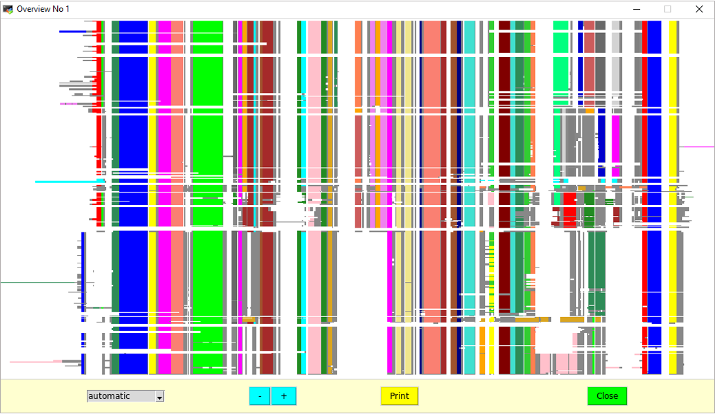 |
In this frame, the alignment is schematized by replacing every residue by a grey pixel over a white background. It is then possible to map any feature on top of this scheme. Clicking anywhere on the scheme will automatically centre the main snapshot window on the corresponding position. On the scheme, a stippled rectangle encompasses the region shown by the main window.
Below the snapshot frame, a control panel allows interaction with the scheme.
The combobox on the left is a feature selector. By default, it is set to 'automatic', meaning that all features drawn or removed in the main window will automatically be drawn or removed in the Overview window. Selecting any feature in the combobox will simply display it on the Overview.
The '+' and '-' buttons will zoom in and out the scheme.
The 'Print' button will output a PNG file of the schematic snapshot in its current state. The user is prompted to give an output file name.
The 'Close' button will close the 'Overview' window.
4.2 Editor
A fruitful exploitation of multiple sequence alignments (MSAs), which ensures high-quality data usage by analysis tools and feature mapping, is directly dependent on the alignment's accuracy. Although research on dedicated alignment algorithms is still intensive and the resulting software is becoming increasingly accurate, the need for manual MSA inspection, curation, and editing remains essential. This is why Ordalie integrates a high-performance sequence editor, inspired by SeqLab from the GCG Wisconsin Package.
Entering the Editor tool will first clear the sequence from any displayed feature and colour the sequences according to physicochemical properties. The default colouring scheme is:
Figure 4:
Amino acids colouring scheme in the Editor
 |
The default scheme can be changed inside the 'Edit -> Preferences' menu item.
| |
|
|
| As the sequences are changing upon edition, some functionalities will not be available in the Editor. |
|
| |
|
At the bottom of the Ordalie window, the Control panel will display the following buttons from left to right:
Figure 5:
The control panel of the Editor tool.
 |
Clears any current sequence selection.
This will group the selected sequences. The names of the grouped sequences will be coloured in a different colour, a unique colour for a given group. If one or more sequences already belong to a group, the user should decide through a dialogue box, if the sequences should be merged with an existing group, or if a new group should be created.
Grouped sequences will behave as a single sequence.
The selected sequences will be removed from any group. If a group consists of only one sequence, the group is automatically destroyed.
By default, only gaps ('. ') can be deleted or inserted, it is not allowed to insert/delete amino acids. Unlocking the sequences allows the insertion/deletion of residues.
“Rem. Col. Gap.” stands for “Remove columns of gaps”. Ordalie runs through all snapshot columns and removes those containing only gaps. A 'Rem. Col. Gap. ' is automatically done when leaving the 'Editor' tool.
This creates a TFA file copy of the current snapshot under edition. The user is asked for a file name the first time, and successive 'Save' will use this file name to output the snapshot.
Leaves the 'Editor' with all the changes made. A dialogue box will ask the user if the current snapshot should be overwritten, or if a new snapshot should be created with the current changes.
Leaves the 'Editor' and restore the original snapshot.
Clicking inside the snapshot frame will show a yellow blinking cursor. The following actions are then available:
- The <Left>, <Right>, <Up> and <Down> arrows move the cursor accordingly.
- <Backspace> deletes the gap/character before the blinking cursor. In lock mode, only gap characters can be deleted.
- <Shift-Right> pushes contiguous characters placed immediately at the right of the blinking cursor up to the next gap character. When dealing with grouped sequences, the next gap is the position which contains a gap for ALL sequences of the group.
- <Shift-Left> pushes contiguous characters placed at the left of the blinking cursor up to the next gap character. When dealing with grouped sequences, the next gap is the position which contains a gap for ALL sequences of the group.
In order to speed up editing, pressing keypad or keyboard digits [0-9] stores the number in a buffer, i.e. pressing '1' then '2' will store number 12 in the buffer. Pressing then the <Left> arrow will move the cursor 12 characters to the left, and will empty the buffer. All the actions previously described can take advantage of this mechanism.
4.3 The Identity tool
This tool is used to query information on identity percentages between sequences or between zones of sequences.
Figure 6:
The control panel of the Identity tool
 .
. |
The identity percentage can be computed for all or some selected sequences and over all or a user defined residue range. The left part of the Control panel deals with sequences and residue range selection.
- Feature : displays the available feature. The user can then select one or more feature items as a residue range.
- Clear : clears all residue ranges and all sequences previously selected.
- Select All : selects residues from the whole snapshot.
The 'Compute' button calculates the identity percentage between selected sequences for the selected residue range. A summary of the computation is logged and is available through the Log console. The selection of two sequences for which the identity percentage is desired is done with the following two comboboxes. The identity percentage and the length of the two ungapped sequences is then given.
The 'Summary' button will make a window appear that will give for the whole sequence and for each group :
- The average identity percentage,
- The standard deviation,
- The pairs having the maximum and minimum identity percentage.
The 'Return' button will leave the Identity tool.
4.4 The Search motif tool
This tool allows the user to search for a particular sequence motif inside the current snapshot.
The syntax of the search pattern follows the rules of the FindPatterns program of the GCG Wisconsin Package [20]. A detailed description of the syntax is available in Appendix 6.2.
Figure 7:
The Control panel of the Search motif tool
 |
The Control panel is limited to the motif entry box in which the pattern should be entered, the 'Search' button to launch the search, the 'Find Next' button to go to the next occurrence of the motif, and the 'Return' button to leave the search tool.
When a motif is found, the background of the snapshot window will become black, and all the instances of the motif will be highlighted in red.
The “search motif” is the only tool that can be called within the “editor” tool.
4.5 The Clustering tool
The 'Clustering' tool allows the creation of clusters (or groups) of sequences based on numerical criterions characterizing the sequences to be clustered. The computation can be done using all or part of the sequence as well as all or part of the snapshot columns. The user chooses one or more numerical criterions as the basis for the computation and a clustering algorithm. The computation can then be launched and the newly created sequence clusters are automatically displayed in the main window. The different clustering trials are temporally kept while using the clustering tool, but a given clustering can be saved as a new snapshot.
At present, the available criterions are:
- Identity percentage : for each sequence, the identity percentage computed over the selected residue range against all other selected sequences.
- Length : the sequence length.
- Hydrophobicity : only available for Macsim alignments.
- Isoelectric point (pI) : the isoelectric point is computed using EMBOSS pKa values for amino acids,
- Amino acid composition : the relative percentage of the 20 amino acids for a given sequence.
Ordalie clusters and automatically defines the number of groups. The clustering algorithms along with the algorithms that define the number of clusters are taken from the Cluspack package. The available methods are:
- kmeans / DPC (Density of Points Clustering) [18]: The clusters identification is done using a point density criteria. The actual cluster selection is done according to the k-means algorithm.
- Hierarchic / Secator [19] : The groups are identified through an ascendant hierarchical classification. The cluster selection is done using an inertia loss criterion.
- Mixture Model [11] / AIC [1] or BIC [12] : After a Gaussian modelling of the data distribution, the clustering is done according to AIC or BIC criteria.
Figure 8:
The control panel of the Clustering tool.
 |
The left part of the Control panel deals with sequence and residue range selection.
- Feature : displays the selected feature. The user can then select one or more items of this feature as a residue range.
- Clear : clears all residue ranges and all sequences previously selected.
- Select All : selects all columns of the current snapshot.
If no sequence names are selected, the clustering will use ALL sequences. If some sequences are selected (more than 3), then the clustering will only apply to these selected sequences. The remaining ones will be kept as a separated group.
The pull-down menu allows the selection of the criteria to be used for the computation. Several criteria can be selected at the same time.
| |
|
|
| The 'Life domain' criterion clusters the sequences into Eukaryota, Archaea, Prokaryota and Other groups. This criterion cannot be associated with another one. |
|
| |
|
The 'Method' pull-down menu permits to choose the algorithm to be used for clustering computation.
- Hierarchic clustering / secator,
- kmeans / DPC (Density of Points Clustering),
- mixture model / AIC criterion,
- mixture model / BIC criterion.
The “Compute” button will launch the computation. The newly computed sequence clusters are directly displayed in the main Ordalie window.
The 'Reset' button will erase any clustering done so far and show the original clustering if any. The 'No Clusters' buttons removes all groups and leaves all the sequences as a single group.
The “Clusters Names” button will pop up a window allowing to give a name to each cluster. This cluster name may be used in subsequent analysis to identify the clusters, like in the “Tree” display, or the “Barcode” tool.
The 'Save' button will leave the clustering tool and the current clustering will be saved. The user is prompted whether to overwrite the current snapshot or to create a new one. The 'Return' button leaves the Clustering tool and displays the snapshot in its original state.
4.6 The Tree tool
The 'Tree' tool can be divided in two part. The first part consists in the tree building, which is done through the main Ordalie window. Once the tree is computed, its exploitation will be done in a dedicated new window.
The tree is computed using the FastME program [9] using default parameters. Ordalie computes first a distance matrix based on identity percentages calculated over the selected residue range. Although Bayesian based algorithms seem to produce more accurate trees, FastME is a good compromise between speed and accuracy.
Figure 9:
The Control panel of the Tree building tool
 |
The left part of the Control panel deals with sequence and residue range selection.
- Feature : displays the selected feature. The user can then select one or more feature items as a residue range.
- Clear : clears all residue ranges and all sequences previously selected.
- Select All : selects residues from the whole alignment.
The following buttons can be used to control the tree computation:
- With PDB seq : includes PDB sequences in the tree computation. By default, Ordalie doesn't use PDB sequences as they are supposed to have their original sequence inside the snapshot.
- Pairwise / global : defines the type of gap removal algorithm to be used. 'Pairwise' (checkbutton on) means that, for each pairs of sequences, positions containing gap are excluded from the computation. 'Global' (checkbutton off) means that only complete columns of residues will be taken to compute the tree.
- Load Tree : it is possible to import a tree file into Ordalie. The tree file should be in a NEXUS format, and the tree leaves identifiers should match all or part of the sequence names present in the snapshot.
- Bootstrap : By setting the 'Bootstrap' checkbutton on, Ordalie will perform <N> bootstraps, N being the number entered in the text field located below the 'Bootstrap' checkbutton. Ordalie pre-computes an ad-hoc value for the bootstrap, the value being equal to 1.1 times the total number of sites used to compute the tree. A loaded tree can also be bootstrapped.
The 'Draw' button launches the computation, and draws the resulting tree in a separate and dedicated window. The 'Return' button leaves the Tree tool.
Each newly computed tree will appear in a new and dedicated window, that allows the exploration of the tree characteristics.
Ordalie can to render two types of trees: dendrograms and radial trees. Some of the following options are specific to one or the other tree representation (see below).
Figure 10:
The Tree rendering window displaying a radial tree. The circles at each node indicate whether the bootstrap value for the node is higher (green) or lower (red) than the defined threshold. The sequences are coloured according to their cluster.
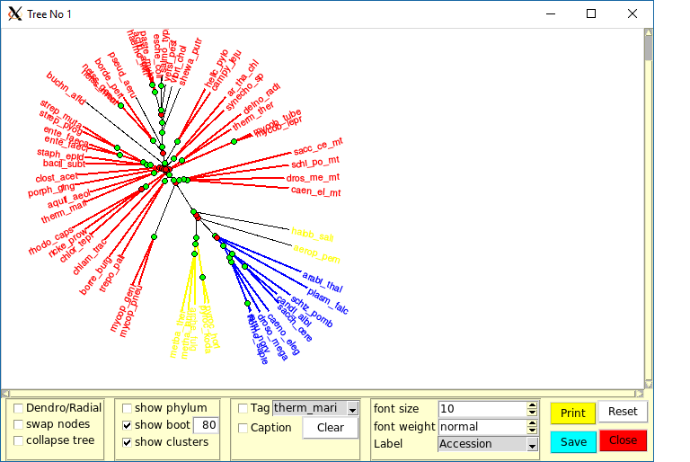 |
The upper part of the tree rendering window is the drawing area, and the bottom part the control panel area.
The drawing area displays the current tree. The tree can be moved in all directions by simply dragging the mouse with <Button-1> down. A radial tree (see below) can be scaled by using the mouse wheel, while using the mouse wheel on a dendrogram will scroll up and down the tree. Finally, a right click <Button-3> will make a contextual menu appear which allows changing the dimensions of the tree. If the tree is a dendrogram, then the branch length and the height separating branches can be changed. If the tree is a radial tree, the tree can be rotated.
The control panel is divided in several parts. From left to right:
General tree options:
- Dendrogram/radial : change the type of tree representation.
- Swap node : when activated, all the nodes of the tree present a little orange disc. By clicking on it, the branches going out from this node are swapped (rotated) around this node.
- Re-root tree (only for dendrogram) : when activated, all the nodes of the tree are marked with a little green disc. Although the tree is an unrooted tree, it is possible to define a new root (the two outmost branches) by clicking on a disc.
Adding information to the tree representation:
- Show Phylum : if the phylum information is available for the sequences, then the sequence names are coloured according to their life domain : eukaryots in red, archaea in blue, bacteria in yellow, and viruses in black.
- Show bootstrap : if the bootstrap computation has been done, each node will display a disc coloured in green or red depending on whether or not its bootstrap value is higher than the threshold (in %) defined in the text field next to the 'show bootstrap' checkbutton (default value 80%). Green circles correspond to boostrap values above the threshold, red circles correspond to values below. In the case of a dendrogram, the absolute value of the bootstrap is also written at each node. In radial tree, pointing the mouse over a disc will display the absolute value of the bootstrap.
- Show clusters : if the snapshot has been clustered, then the branches of the tree will be coloured according to the group they belong to.
Tags and tree annotation:
- Tag : the leaf specified in the combobox aside the checkbutton 'Tag' will be surrounded by a thick black box. This allows the quick identification of a sequence in case of a furnished tree.
- Caption : this will add a caption to the tree. The first time this option is invoked, or if the 'Clear' button is pressed, a window will appear to let the user customize the caption.
Leaf labels:
- Font size : changes the size of the font used to display labels (sequence names).
- Font weight : changes the font between normal and bold.
- Label : defines the 'text' to be displayed as leaf labels which is by default the sequence name. It may be useful to show the accession number, or the accession number with the species, etc ...
Buttons:
- Print : makes a PNG file of the current state of the tree.
- Reset : resets the tree to its original configuration.
- Close : closes the window.
4.7 The Conservation tool
Traces of the evolution pressure that maintains the structure and function of a protein family can be found while examining the residue conservation along the snapshot. Both global and group conservations may help in deciphering functional sites like binding sites, interaction patches, or specialization coupled with intra-groups organization.
Ordalie offers several methods to compute conservation. Within this tool the user can try several methods to compute residue conservation. The results are temporarily kept until they are saved. A saved residue conservation computation becomes then a new feature attached to the current snapshot and can, as any other feature, be used in any tool allowing feature display.
Many methods exist to compute conservation, and they have been tested and compared extensively [17,4]. Ordalie implements some of them, as well as two home-made conservation methods.
This method is essentially a counting method. Different levels of conservation are defined thanks to two pre-set thresholds. At a global level, a column with 100% conserved residues (the 'identity threshold') is assigned to 'identity conservation'. A column with at least 80% conservation (the 'global threshold') is considered a 'conserved' column. Within a group, however, only 'identity conservation' is considered. The thresholds can be changed through the 'Preferences' menu.
In these methods, only columns containing more than 5 residues are considered, and the computation proceeds through two steps. First, all the columns are scored with the chosen method. In a second step the columns with their associated scores are clustered, and the clusters are ranked according to their mean conservation scores. The two clusters containing the highest scores are considered to contain the columns corresponding to 'strictly conserved' and 'globally conserved' residues. The same computation is repeated for each group, but only the cluster with the highest scores is taken.
The available automatic methods are:
- BILD : Bayesian inferred score, see [2],
- Liu : taken from Liu et al. [10]
- Mean Distances : the algorithm implemented in ClustalX [13]
- Vector Norm : this method uses a physicochemical representation of amino acids based on their volume and polarity. The score is proportional to the most present amino acid in the column. The method is described in detail in the Appendix 6.3.
- Multi : each column is scored using several scores (here the 'Vector norm' and 'Mean Distance' scores) before being clustered.
Figure 11:
The control panel of the Conservation tool
 |
From left to right in the Control panel:
- Method : the scoring method to be used.
- Title : an optional title for the ongoing conservation calculation can be added.
- Include PDB : by default, the conservation calculation does not include PDB sequences as their genomic sequence is usually also included in the snapshot.
- Only global : if checked, the conservation will only be performed for the whole snapshot, conservation inside groups will be discarded.
- Compute : launches the computation.
- Show : Each computed score is saved temporarily and can be recalled using this combobox. By default, the score is called 'tmp<Method>-<x>' where <Method> is the method used and <x> an index. If the score is saved, its name will change to '<Method>-<x>'.
- Show scores : opens the Scores frame just below the alignment and displays the scores as a graph. The drawn scores correspond to the scores currently selected.
- Save : save the current score (the score indicated in the 'Show score' combobox) along with its 'Title'. The saved score name will be changed in that combobox, and the score will appear as a new feature in the 'Normal' mode.
- Return : returns to the 'Normal' mode.
4.8 The Superposition tool
One of the strengths of Ordalie resides in its ability to link/map features to the 3D models (when available) of proteins. To exploit at best the feature mapping it is essential to proceed in the scope of the structural differences observed between proteins. To achieve that, Ordalie can superpose the structure according to feature, and/or user defined residue range.
A protein structure can be made of several chains, which may be identical or not. A chain is usually composed of an amino acid polymer and ligands (in Ordalie, water molecules are considered as ligands). It is important here to understand that, although superposition computation are done using the polymer sequences, the entities that are moved (superposed) in Ordalie are the entire chains.
| |
|
|
| When applying a superposition to a chain, all residues of this chain (polymer AND ligands) are moved. |
|
| |
|
The chain superposition is done in three steps:
- Selection of the superposition zone. Depending on the structure, the zones may consist of an entire domain, or of selected secondary structures, for example.
- Selection of the superposition zones. Depending on the structure, the zones may consist in a domain, or some selected seconddary structures for example.
- Selection of the chains that would be superposed.
- Selection, between the chains selected for superposition, of the reference chain. The reference chain will not move, all the other selected chains will be superposed onto it.
The detailed superposition algorithm is presented in Appendix 6.5.
Figure 12:
The Control panel of the Superposition tool.
 |
From left to right the superposition Control panel is made of:
- Features : display the selected feature. The user can then select a feature item as a residue range.
- Clear : clears all residue ranges and all sequences previously selected.
- Select All : selects residue from the whole snapshot.
- All Helices : selects all helices present in the sequences.
- All Strands : selects all -strands present in the sequences.
| |
|
|
| The 'All Helices' and 'All Strands' selections will take, for each secondary structure type position, the minimal common part of all existing secondary structures present at that position. |
|
| |
|
- Superpose : launches the superposition. As mentioned previously, this will be done in two steps:
- Open the chain selection window where the user should select all the chains concerned by the current superposition.
- When done, the Reference chain window will open to choose the reference chain (the non-moving chain) among the previously selected chains.
- Display : opens the 3D Viewer (see the 3D Viewer section for details 4.9).
- Return : leaves the superposition tool.
Suppose the loaded alignment concerns a protein known to be a homo-dimer (an  structure) under biological conditions, and for which several 3D structures of some proteins coming from different organism have been solved. By investigating PDB ID (say 1abc and 1def), it is also known that all structures are made of two chains, A and B. The build alignment contains the corresponding sequences PDB_1abc_A and PDB_1def_A.
When loading the alignment, Ordalie will recognize the two PDB ID through their sequence names PDB_1abc_A and PDB_1def_A and will then download from the PDB website the two structures with atomic coordinates, and store them inside a dedicated database. Note that Ordalie knows the coordinates for all the atoms of ALL chains of the structure, not only chain A.
Several cases may be encountered when performing a superposition:
The snapshot contains the sequence named PDB_1abc_A and PDB_1def_A. When superposing PDB_1def_A on PDB_1abc_A, only atoms of 1def chain A will change. Thus in the 3D Viewer, the whole structure of 1abc will be correct (its the non moving molecule), and 1def will have chain A on top of 1abc chain A, and 1def chain B somewhere in space. The symetry of the dimer is broken, as only chain A as moved.
Ordalie doesn't know anything about monomers, dimers, multimers in general. It is up to the user to provide the information, by giving Ordalie the sequences of the chains of interest.
| |
|
|
| To manipulate a multimer in Ordalie, all the sequences corresponding to the chains of the reference AND the sequences of the chains of the target structure should be present in the alignment. |
|
| |
|
If the alignment contains PDB_1abc_A, PDB_1abc_B, and PDB_1def_A, PDB_1def_B, it is then possible to superpose the two dimers. A first superposition step where only PDB_1abc_A and PDB_1def_A are selected will bring PDB_1def_A on top of PDB_1abc_A. A second superposition step where only PDB_1abc_B and PDB_1def_B are selected will bring PDB_1def_B on top of PDB_1abc_B.
4.9 The 3D Viewer tool
The 3D Viewer is one of the most useful tool in Ordalie. Although it does not offer all the features and functionalities that would a proper Molecular Visualization program like VMD or PyMol would do, it can be of great help in understanding protein features in the framework of protein structures.
The Ordalie 3D Viewer is organized around the 'Molecule' and 'Object' notions. A 'Molecule' consists in all the chains (and consequently residues and atoms) that are present in a given PDB entry. An 'Object' belongs to a Molecule, and can be a composition of several elements (full chains, parts of chain, residues, ligands, etc... ) belonging to that molecule. Objects can be painted with several colours and can contain several kinds of representation. Feature mapping only applies to objects.
By default, Ordalie will create 3 objects per molecule:
- AL<molecule name><chain> which is a stick representation of all the atoms of the chain,
- CT<molecule name><chain> which is the C(or phosphate) trace of the chain,
- CA<molecule name><chain> which is the ribbon representation of the chain.
At present, Ordalie does not handle hydrogen atoms.
Ordalie is able to represent a structure in several ways.
- Ribbon : the C/P smoothed ribbon. By default, the path atoms are the Ca and P for amino acids and nucleic acids respectively.
- Ca/P trace : a simple link between Ca or P atoms.
- CPK : each atom is represented as a sphere whose radius is the VDW radius of the atom.
- Pearl : the residue is simply represented by a solid sphere placed at the centre of mass of the residue.
- Atoms : a wireframe representation. Standard residues are drawn according to their topology. All other compounds (modified residues, ligands, ...) will be drawn according to a distances criteria. Depending on the quality of the structure, this may lead to chemically wrong atomic bonds.
The 3D Viewer window can be divided in 4 parts. The top of the window is used to display information about picked atoms. Below is the 'Quick Mapping' panel. Below this panel, from left to right are the 'Molecular Objects' frame, the main 3D window, and the 'Actions' panel at the right. The 3D window can be maximized by hitting the <F1> on the keyboard, and hitting <F1> again gives the window its original geometry. All panels may be switched on or off by hitting the <F2> key.
The four comboboxes of this panel allow making a quick mapping of features on a given molecular object. The left outmost combobox selects the molecule, then the object onto which the feature will be mapped. There are then two features selectors. It is possible to map two features on a same object by selecting one feature with 'Feature 1' combobox, and a second feature with the 'Feature 2' combobox. The features are drawn in order, feature 1 before feature 2. Care should be taken when selecting Feature 1 and Feature 2 as Feature 2 can completely cover Feature 1. For example, if Feature 1 is set to conservation, which implies residues colouring, and Feature 2 is set to PFAM-A, a lot of conservation won't be seen as a PFAM domain extends to a large range of residues. In this case, Feature 1 should be set to PFAM, and Feature 2 to conservation.
Below the 'All On' and 'All Off' buttons that switch on and off all objects that have been defined in all Molecules is the list of all 3D molecules present in the snapshot. Aside the molecule name is the 'New' button that allows the definition of new objects for that molecule (see section 'Object Editor' 4.9.4 below). Clicking on a molecule name will open/close the list of the objects defined for that molecule. An object coloured in green is switched on and is displayed on the screen, a red object name means the object is switch off. Each object name is followed by the 'Edit' and 'Del' buttons, used to redefine and delete the object respectively.
This window contains the 3D objects themselves. The objects can be manipulated by the mouse through an arcball system, that is a virtual trackball. All the objects of the scene are enclosed in a sphere, and the objects are moved by dragging the sphere up and down and left to right using mouse Button-1, the mouse mimics the hand that would roll the sphere. The mouse wheel is used to zoom in and out the scene. A right drag with <Button-3> will translate the scene in the x-y plane. A <Control-B1> click will show the label of the atom being below the mouse pointer.
Although the Ordalie 3D Viewer tool is not intended to be a complete Molecular graphics program, it still offers some functionalities which are, from top to bottom:
- Reset : cancels all ongoing actions (for example, distance definition),
- Clear Ids : switches off all atom labels,
- Clear Distances : switches off all distances,
- Distances : computes the distance between two picked atoms,
- Centre On Atom : the picked atom becomes the rotation centre of the scene,
- Print : outputs a PS file of the scene,
- Full Screen : toggles the window into a full screen window,
- Stereo : not yet available,
- Close : closes the 3D Viewer window.
4.9.4 The Object Editor
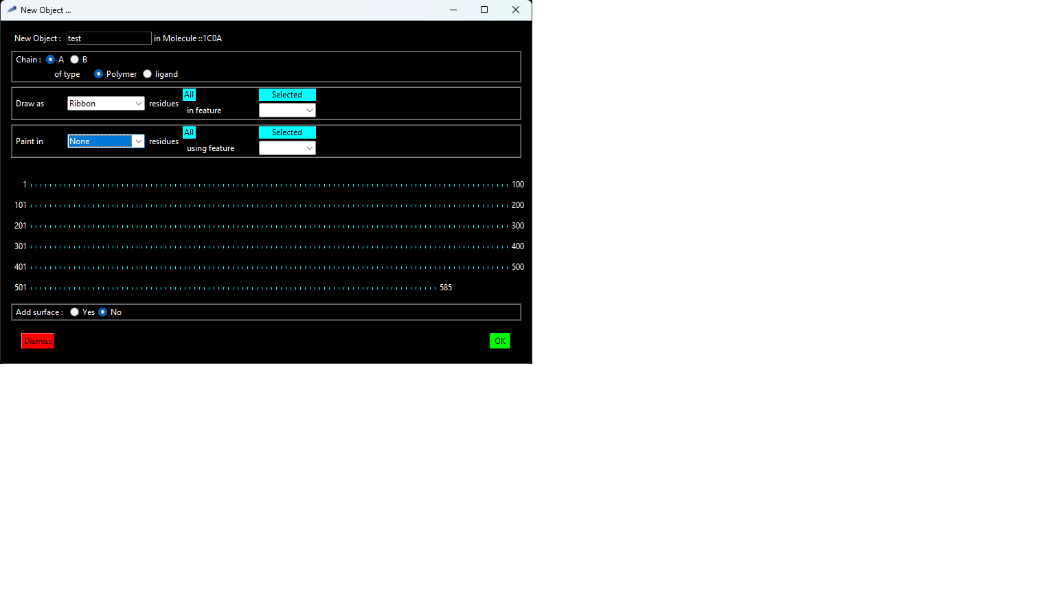
An object is an ensemble of residues and/or ligands belonging to one or several chains, and displayed in given styles with given colours. The Object Editor can be invoked to create a new object (the 'New' button) or to edit an existing object (the 'Edit' button).
Figure 13:
The 3D object creation window.
|
|
In case of a new object creation, the new object name should be entered in the top entry box. Two objects can not have the same name.
The object edition can then be done in a five-step process:
- select the chain of interest and the type of residues in the chain : polymer residues (amino acids or nucleotides) or the ligands,
- select a representation type,
- select residues onto which to apply the selected style,
- select a colour,
- select residues onto which to apply the selected colour.
This process is iterated until all pieces of the object are set up.
Finally, it is possible to add the molecular surface surrounding the object atoms by checking the checkbox at the bottom of the object window.
When applying a colour or a representation style, the user should specify the residues it should apply to. There are three ways to do so:
- the 'All' button will select all the residues of the current chain. This may be useful to give all residues the same colour for example.
- The 'Selected' button : this refers to residues which have been selected with the mouse onto the residue frame. In this frame, clicking and dragging the mouse with <Button-1> down will select a range of residues.
- The 'Feature' combobox : this will select residues corresponding to the selected feature.
The object is then finished by clicking on the 'OK' button. The new object will be added to the object list on the corresponding molecule.
4.10 The Features Editor
This tool is dedicated to feature management, feature creation, deletion and edition.
The Control panel of the 'Features Editor' is really simple.
Figure 14:
The Control panel of the Feature Editor tool
 |
It consists, from left to right, in:
- Features : displays the selected feature. The user can then select a feature item as a residue range.
- Clear Selection : clears all residue ranges and all sequences previously selected.
- Delete feature : This will delete the current feature for all sequences.
- Load Feat. File : loads a file containing user-defined features. The feature file format is described in Appendix 6.4.
- Features Summary : launches the Features summary tool which allows an overview of any feature within the snapshot. See section 4.11.
- Save : saves the feature changes and returns to the 'Normal' mode
- Return : returns to the 'Normal' mode and restores original features.
It is important to understand the difference between a Feature and an Item of a Feature. Here, a Feature represents a set of instances of a given sequence characteristic that may be distributed over the whole snapshot. A Feature Item, or Item for short, is one instance of a Feature for a given sequence at a given place in the snapshot.
Contrary to all other tools, it is possible to interact directly with the features inside the snapshot window. A right click makes a contextual menu pop up, allowing several actions.
| |
|
|
In the 'Feature Editor' tool, action of <Button-1> is changed through key combination :
<Button-1> alone : the action applies to the sequence under the mouse pointer.
<Control + B1> : the action applies to the group the sequence pointed by the mouse belongs to.
<Shift + B1> : the action applies to all the sequences present in the snapshot. |
|
| |
|
Selects the Item just under the mouse pointer. If only <Button-1> is pressed, then the Item of the sequence will be selected, if <Control + B1> is pressed then all the Items at that position for sequences of the group will be selected, and if <Shift + B1> is pressed all Items appearing at that position for all sequences in the snapshot will be selected.
Selects all Items of a sequence, a group of sequence or the whole snapshot depending on the key pressed.
| |
|
|
| Selecting all Items for all sequences means that the whole Feature is selected. If it is subsequently deleted, then the whole feature will be deleted. |
|
| |
|
A region (i.e., a residue range) can be selected by pressing and holding <Button-1> and then dragging the mouse along the sequence axis. Depending on whether no key, the <Control> key, or the <Shift> key is held down, the selected region will cover the current sequence, the sequence group, or all sequences respectively. The selected region can then be used to define a new Item.
Clears all selections currently set.
After having selected Items(s) or region, several options are then available.
If the selection refers to one or several already existing Items, it is possible to change some of their properties:
- the residue range of the selected Items can only be changed if they refer to only one zone,
- the Item Colour,
- the Item Score,
- the Item Note.
This option will make a window appear, allowing the description of the new item. If the 'Feature Name' entry is filled with an already existing feature, then the new item will be added to the item list of that feature. If the 'Feature Name' does not exist, a new feature is then created. In all cases the user is supposed to give to the item at least a Colour and optionally a Score and a Note.
This will delete the selected items from the current feature. Note that if all Items of a Feature have been selected, then this option will delete the Feature itself.
The Selected Items will be propagated to all the sequences of the group they belong to. If an Item to be propagated is already present in one or more sequence of the group, the Item will not be propagated.
This will propagate the selected Items to all the sequences of the SNAPSHOT. If an Item to be propagated is already present in one or more sequence of the group, the Item will not be propagated.
4.11 The Features Summary
This representation can render several selected sequences and features on the same page. The sequences are not schematized as in the Snapshot Overview representation, but are shown as they appear in the alignment window.
Figure 15:
The Features Summary window, with the Drawing Area at the top and the Control panel at the bottom
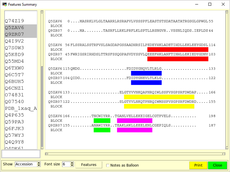 |
The top of the 'Features Summary' window is made of a listbox containing the sequence names on the left, and a drawing area on the right. Clicking on a name selects or unselects the corresponding sequence. Multiple sequences can be selected by holding the <Control> key down while clicking on their names with the mouse.
In the drawing area, for each sequence the sequence ID is written on the left, followed by the position of the first residue in the current sequence line, the amino acid sequence itself as present in the alignment, and the position of the last residue in the line. When a feature is selected, each sequence line is followed by a feature line, with the feature name beneath the sequence ID, and rectangles below sequence positions where the feature is present.
The Features Summary can be moved around by dragging the mouse while holding <Button-1>.
Below the Drawing Area is the Control panel. On the left is a spinbox that selects the type of name the sequence should be referenced with, i.e. its sequence name, its accession number or its bank ID, when available. This choice applies in both the listbox and the drawing area. Follows the font size selector, and then the 'Features' selector. Any number of features can be selected by checking the button corresponding to the desired feature. The 'Notes as Balloon' checkbutton renders or not the note attached to each feature as a flying balloon when the mouse pointer is over the feature. The 'Print' button will ask for a file name that will contain a PNG image of the current drawing area, and the window will disappear by clicking the 'Close' window.
4.12 The Annotation tool
This tool allows adding, modifying and removing “memo tags” anywhere on the snapshot. They can be displayed on or off at any time using the “Annotation” button on the snapshot bar.
A memo tag has three characteristics: its position and size, its colour, and the text note attached to it. The user can use them to annotate a piece of snapshot that will have to be manually re-aligned, to annotate a particular conserved zone of interest for example. The colour can be used as a classification mean, pink for structural annotation, cyan for sequence features, etc...
The Control Panel is fairly simple and is composed from left to right:
- “Show annotation coloured in” can be used to show a given coloured annotation,
- “Show all” will display all available annotation
- “Hide all” will remove all annotation of the screen,
- “Dismiss” will leave the tool,
- “Return” will leave and save all changes made in the annotations.
Annotation creation makes use of the mouse. Table 3 shows the actions associated with mouse button combined with keyboard.
Table 3:
Keys combination for annotation management
| Keys |
Action |
|---|
| <Button-1> |
Select the origin of a new annotation. |
| <Button-1 dragging> |
Define the area of the current annotation |
| <Button-1 release> |
Finish the annotation zone definition |
| <Control> + <Button-1> |
Delete the annotation below the mouse pointer |
| <Shift> + <Button-1> |
Edit the annotation below the mouse pointer |
|
After creating an annotation zone (button-1 released), a window will pop up allowing the user to select the annotation colour and the associated text. The same window appears to edit a given annotation. Clicking <Return> will save all the changes made in annotations.
4.13 Barcode
The “Barcode” tool is another schematic representation of a snapshot. Figure 16 shows an example.
Figure 16:
The barcode window
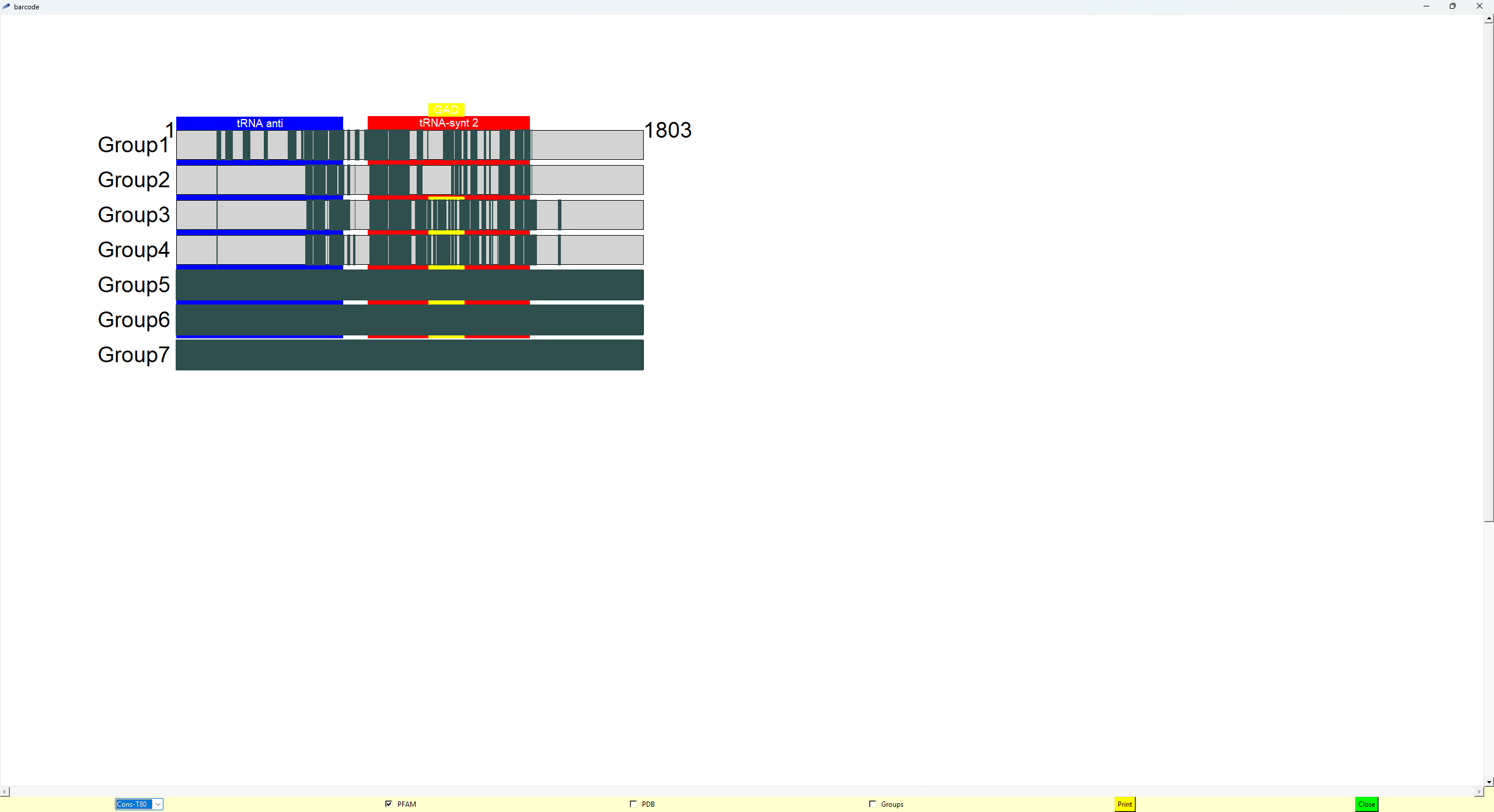 |
The upper frame of the tool is the drawing area. For each group of sequence of the snapshot a lane will be drawn